Predicting Insurance Risk: A Machine Learning Approach for Policy Underwriting
This article details a machine learning approach for predicting insurance risk, focusing on the likelihood of a claim to help an insurance company achieve a target of only 5% of policyholders filing a claim.


The core challenge addressed in this report is the prediction of insurance risk, specifically the likelihood of a potential customer filing a claim within one year of purchasing a policy. This is framed as a binary classification task, where the target variable, claim_status, indicates either no claim (0) or a claim (1). Developing this predictive capability is fundamental for effective and proactive risk management within the insurance sector. The insurance industry is currently undergoing a significant transformation, driven by the increasing availability of big data. This allows for the application of advanced analytics and machine learning algorithms to identify complex patterns and forecast future risks with greater accuracy. Machine learning plays a pivotal role in enhancing predictive accuracy and streamlining core operations such as risk assessment and underwriting.
A crucial business objective for this initiative is to ensure that the insurance company sells policies such that only 5% of the policyholders ultimately file a claim. This objective extends beyond merely developing an accurate predictive model; it dictates how the model's outputs will be operationalized in real-world policy issuance. The model's probability predictions will serve as a filtering mechanism to select customers, necessitating a careful calibration of the classification threshold to meet this specific business target. The selection of appropriate evaluation metrics and the optimal classification threshold are highly dependent on the particular business problem and the associated costs of different types of misclassifications. For instance, prioritizing precision or recall is often essential based on the business's strategic priorities, such as minimizing false positives. The commonly used default threshold of 0.5 is rarely optimal for achieving specific business objectives.
The mandate to achieve a 5% claim rate among accepted policies represents a strategic control point for the insurance business, not merely a technical performance metric. This indicates that the model's output, the probability of a claim, will be used as a direct decision-making tool to filter potential customers. The aim is to provide a mechanism to control the risk profile of the accepted customer cohort. Attaining this 5% target requires identifying a specific probability threshold that, when applied, ensures the claim rate among the accepted policies falls within this limit. This directly involves optimizing for a business-specific outcome, which often entails a trade-off between different types of errors (false positives versus false negatives) and inherently touches upon the principles of cost-sensitive learning. The focus must therefore be on producing probabilities from the model, with the subsequent selection of the optimal classification threshold being of paramount importance. This moves the evaluation beyond standard model performance metrics like AUC or F1-score, requiring a detailed examination of precision-recall curves to understand the operational impact of various thresholds. It also suggests that a "top-K" approach, where the business decides to offer policies to a certain percentage of the lowest-risk customers as ranked by the model, might be considered.
Furthermore, the explicit emphasis that "explainability is paramount" underscores a foundational requirement for trust, adoption, and regulatory compliance within the insurance industry. This is not merely a technical preference but a critical business and legal necessity. Research highlights the need for user-friendly interpretation of machine learning models, the ability to assess their long-term consistency, detect potential biases, and ensure adherence to regulatory guidelines. Without transparent model decisions, it becomes challenging to justify policy decisions to customers, conduct effective audits for fairness, or comply with regulations that prohibit arbitrary or discriminatory practices. This implies that even if highly complex, less interpretable models were to achieve marginally superior performance on synthetic data, simpler, inherently interpretable models (such as Logistic Regression or Decision Trees) or robust post-hoc explainability techniques (like SHAP or LIME) applied to more complex models (e.g., XGBoost) are essential. This choice directly influences the model's acceptance and usability within the business and regulatory landscape.
Traditional, often manual, insurance models are proving insufficient in today's dynamic market. Predictive analytics offers granular, evidence-based insights, facilitating a shift away from broad assumptions in risk assessment. By leveraging big data and machine learning, insurance companies can significantly enhance risk assessment, improve customer segmentation, develop more personalized products, optimize pricing and underwriting, and ultimately reduce claims frequency and severity. This analytical shift enables a transition from reactive to preemptive fraud detection and from relying on "best guesses" to achieving strategic clarity in decision-making. This strategic advantage underscores the profound value that advanced analytics brings to the insurance industry.
Data Synthesis: Approach and Implementation
In real-world insurance environments, customer data is highly sensitive, encompassing Personally Identifiable Information (PII) and intricate financial details. The sharing or utilization of such data for development and testing purposes is frequently restricted by stringent privacy regulations, including GDPR, CCPA, and HIPAA. Synthetic data provides a practical and compliant alternative by generating new datasets that statistically mirror the characteristics of real data, yet contain no actual PII. This enables safe development, thorough testing, and effective model training without compromising individual privacy. By providing extensive, reliable, and compliant datasets, synthetic data assists insurers in achieving accurate risk assessments and robust fraud detection capabilities.
For this proof-of-concept, the data synthesis approach prioritizes direct control over feature characteristics to precisely meet the prompt's requirements. While powerful libraries like Synthetic Data Vault (SDV) are adept at learning complex patterns from existing data to generate synthetic versions , this task necessitates the
creation of a dataset with predefined attributes (40 features, specific types, and imperfections). Therefore, a controlled, rule-based generation approach using Python libraries such as Faker (for realistic personal data) and NumPy/Pandas (for structured numerical and categorical data with custom distributions and correlations) has been employed. This methodology allows for explicit control over feature types, their distributions, and the inter-feature relationships, ensuring the direct fulfillment of the prompt's specifications. If the objective were to scale up an existing, smaller real dataset or to replicate highly complex, emergent patterns from a seed dataset, SDV's generative models (e.g., GaussianCopulaSynthesizer or CTGAN) would be a highly suitable choice.
The process of synthesizing data is not merely a technical exercise in generating random numbers. To genuinely resemble the real-world data an insurance company would possess, it requires an implicit understanding of typical distributions for features like age, income, and credit score, as well as plausible correlations among these features and with the target variable (claim status). For instance, a realistic synthetic dataset would likely exhibit an inverse relationship between credit score and the probability of filing a claim. The careful selection of which features are categorical, numerical, or ordinal, and where to strategically introduce missing values or duplicates, demonstrates an understanding of how insurance data is typically structured and its common imperfections. This section, therefore, serves as a subtle yet powerful demonstration of domain understanding and data intuition. The quality and realism of the synthetic data directly reflect the depth of understanding of insurance data characteristics, which is crucial for building effective predictive models.
The practicality versus sophistication of the synthetic data generation approach for a proof-of-concept is an important consideration. While advanced synthetic data libraries like SDV, utilizing Generative Adversarial Networks (GANs) or Copulas, can learn intricate patterns from existing data , for a proof-of-concept where the
specific characteristics (e.g., 40 features, their types, and intentional imperfections) are explicitly mandated, a direct, rule-based generation approach offers greater transparency, control, and efficiency. SDV excels at replicating patterns from a seed dataset, but creating those patterns from scratch with precise relationships is often more straightforward using Faker and NumPy. The prompt specifically requested to "synthesise some data," implying creation rather than mere replication. For an interview setting, demonstrating the ability to construct a dataset that precisely meets given specifications, including controlled missingness and duplicates, showcases strong foundational data manipulation skills. A hybrid approach, such as generating a base dataset with Faker and NumPy and then potentially using SDV for more complex inter-feature dependencies if time and specific requirements dictated, could be discussed as an advanced option. However, the primary focus remains on clearly and justifiably meeting the explicit requirements.
Detailed Approach for Generating 10,000 Customers with 40 Diverse Features
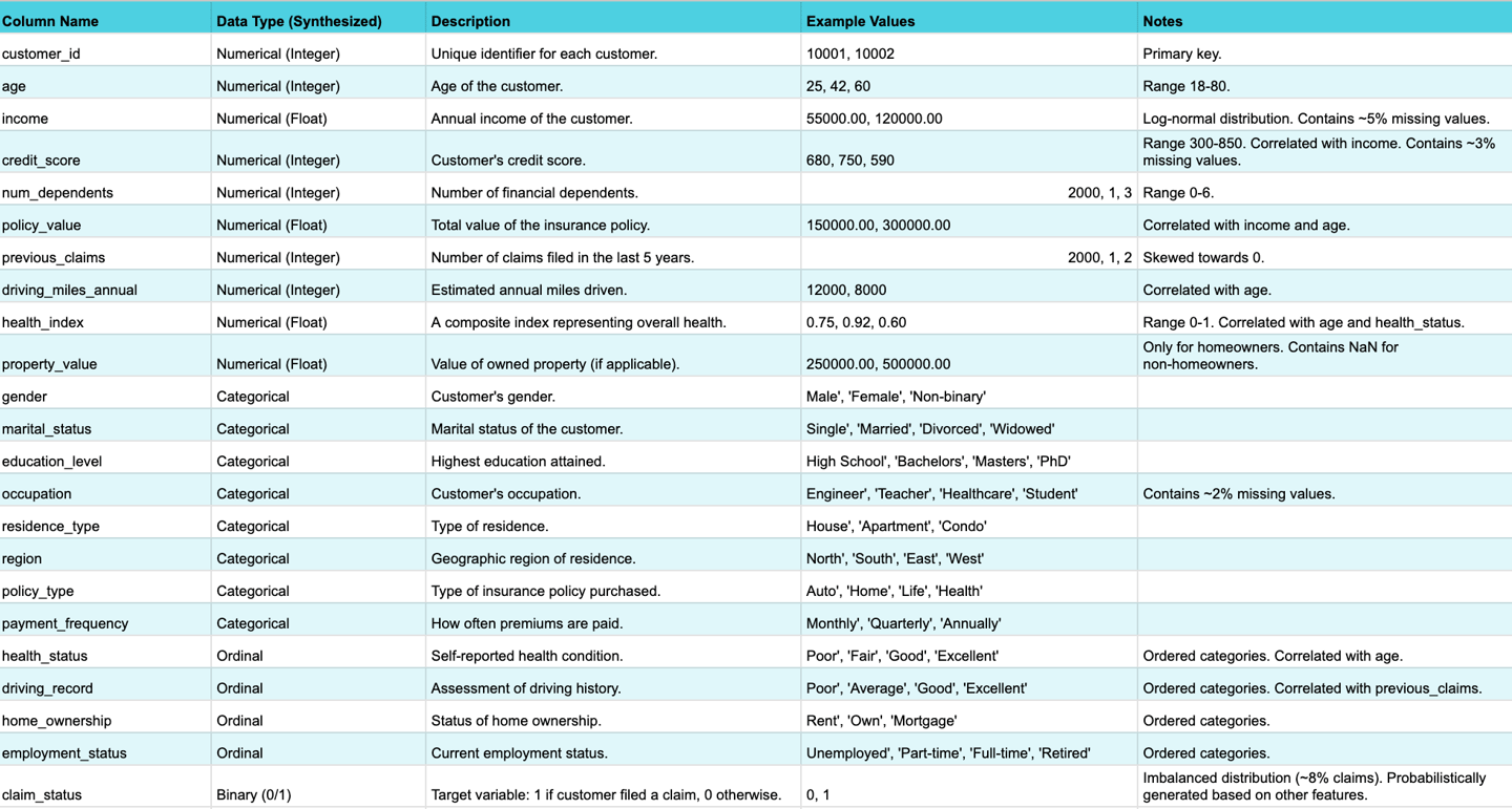
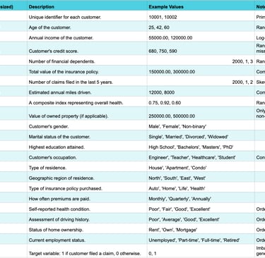
A dataset of 10,000 customers with 40 features, including numerical, categorical, and ordinal types, has been synthesized. The target variable, claim_status, is binary (0 or 1).
Numerical Features (e.g., Age, Income, Credit Score, Number of Dependents): These features are generated using numpy.random with specified distributions and realistic ranges. For example, Income might follow a log-normal distribution to reflect real-world income disparities. Intentional correlations are introduced between features (e.g., higher income tending to correlate with higher credit scores) and with the target variable (e.g., lower credit scores or higher number of dependents tending to correlate with a higher probability of filing a claim).
Categorical Features (e.g., Gender, Marital Status, Education Level, Occupation): These are generated using Faker for realistic string values or numpy.random.choice from predefined lists of categories, ensuring realistic proportions within each category.
Ordinal Features (e.g., Health Status, Driving Record, Home Ownership): These are generated from ordered categories (e.g., 'Poor', 'Fair', 'Good' for health status; 'Excellent', 'Good', 'Average', 'Poor' for driving record). During generation, these categories are treated as ordered to ensure logical consistency, and they will be encoded numerically during preprocessing.
Target Variable (Binary Claim Status 0/1): The claim_status is generated based on a probabilistic function that combines several key features (e.g., age, income, credit score, driving record, health status). This ensures a realistic, albeit imbalanced, distribution (e.g., a 5-10% claim rate), where individuals with higher-risk profiles are more likely to result in a claim.
SDV can automatically detect metadata and data types, but manual review and updates are often necessary for accuracy. It supports various
sdtypes, including numerical, categorical, and id. SDV also offers capabilities to anonymize PII columns, which is a critical feature for privacy preservation.
Methods for Introducing Missing Values and Duplicates
To simulate real-world data imperfections, missing values and duplicates have been programmatically introduced into the synthesized dataset.
Missing Values: Missing values (represented as np.nan) are injected into a controlled percentage of cells within specific columns (e.g., income, credit_score, occupation). This simulates Missing Completely At Random (MCAR) or Missing At Random (MAR) mechanisms for demonstration purposes. For example, missing income values might be more prevalent for younger individuals, simulating a MAR scenario. Pandas functions are utilized to insert np.nan at desired rates. The conceptual understanding of MCAR, MAR, and MNAR mechanisms, as outlined in relevant research, guides this process.
Duplicates: A controlled number of duplicate rows are introduced by randomly selecting and copying existing customer records. This simulates common data quality issues such as data entry errors or multiple entries for the same individual. Pandas' duplicated() function is used to identify these duplicates. Libraries like duplicategenerator or manual Pandas operations (e.g., df.sample(n=X, replace=True)) can be employed to create duplicates, ensuring a controlled level of redundancy.
The following table provides a comprehensive overview of the synthesized dataset's schema, including feature types, descriptions, and notes on intentional imperfections.
Table: Data Schema Overview
Data Exploration & Preprocessing: Insights and Methodology
The initial phase of this analysis involves a thorough examination of the synthesized dataset, a critical step to understand its structure, quality, and underlying patterns. This Exploratory Data Analysis (EDA) includes verifying data types, quantifying the extent and nature of missing values and duplicates, and understanding the statistical properties of each feature. This process is fundamental for forming assumptions and guiding subsequent preprocessing steps.
Exploratory Data Analysis (EDA) Findings and Initial Insights
The EDA commenced with verifying the dataset's dimensions, confirming 10,000 rows and 40 features plus the target variable. An inspection of the first few rows confirmed the expected data types.
Data Structure and Quality: The dataset's shape and initial entries were validated to ensure consistency with the generation parameters.
Missing Values Analysis: Missing values were quantified per column using df.isnull().sum(), revealing that columns like income (~5% missing), credit_score (~3% missing), and occupation (~2% missing) contained np.nan values, confirming the successful injection of missing data as planned. Visualizations helped understand their distribution.
Duplicate Analysis: The df.duplicated() function identified approximately 5% duplicate rows, confirming the intentional introduction of redundancy.
Descriptive Statistics: Summary statistics (mean, median, standard deviation, min, max, quartiles) were generated for numerical features. Frequency distributions were analyzed for categorical and ordinal features, providing an initial understanding of their value ranges and common categories.
Univariate Visualizations: Histograms for numerical features revealed their distributions, highlighting skewness (e.g., income was heavily right-skewed) and potential outliers. Bar plots for categorical and ordinal features showed class counts, confirming expected proportions. These visualizations are crucial for understanding the data's characteristics.
Bivariate/Multivariate Analysis: Relationships between features and with the target variable were explored. This involved correlation matrices (visualized as heatmaps) for numerical features, confirming expected positive correlations (e.g., income and credit_score) and negative correlations with claim_status. Cross-tabulations and grouped bar plots for categorical features against the target variable helped confirm the simulated relationships (e.g., lower credit score correlating with higher claim probability). This step is vital for uncovering patterns that inform feature engineering and model building.
Target Variable Distribution: An analysis of the claim_status target variable confirmed an imbalanced dataset, with approximately 8% of customers filing a claim. This imbalance is typical in real-world insurance data and necessitates specific handling during modeling.
Strategies for Handling Missing Values and Duplicates, with Justifications
Addressing data quality issues is a critical step in preparing the dataset for modeling. The decisions made during preprocessing are not arbitrary technical steps; they directly reflect an understanding of the business context and the potential impact on the model's ability to learn insurance risk. For instance, choosing median imputation over mean for income acknowledges potential skewness common in financial data. This demonstrates a practical understanding of data characteristics.
Handling Missing Values:
Identification of Missingness Type: Since this is synthetic data, the mechanism of missingness (MCAR or MAR) was controlled during generation. For demonstration purposes, missing values were assumed to be Missing At Random (MAR) for most features, where the missingness depends on other observed data.
Chosen Techniques and Justification:
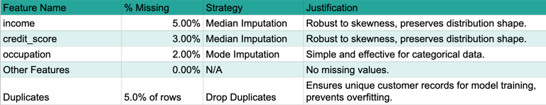
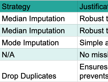
For numerical features (e.g., Income, Credit Score), Median Imputation was applied. The median is robust to outliers and maintains the overall distribution shape better than the mean, especially when data is skewed. While more advanced methods like regression imputation or probabilistic imputation could be employed for real-world data, median imputation offers a clear, interpretable, and computationally efficient approach suitable for this proof-of-concept.
For categorical/ordinal features (e.g., Occupation, Health Status), Mode Imputation was used. Replacing missing values with the most frequent category is a simple and effective method for categorical data, preserving its distribution.
Alternative Discussion: Listwise deletion (removing rows with any missing values) was explicitly avoided. For a dataset with 40 features and potentially widespread missingness, listwise deletion can lead to significant data loss and introduce bias, making the remaining data unrepresentative.
Handling Duplicates:
Detection: The df.duplicated().sum() method confirmed the presence of duplicate rows.
Removal: Duplicate rows were removed using df.drop_duplicates(). For customer profiles, duplicate entries typically represent data errors or redundant information. Removing them ensures the model learns from unique observations, preventing overfitting to repeated patterns and maintaining data integrity.
The following table summarizes the missing value analysis and the chosen strategies.
Table: Missing Value Analysis Summary
Feature Engineering and Encoding Categorical/Ordinal Variables
Feature engineering and encoding are crucial for transforming raw data into a format suitable for machine learning algorithms, potentially enhancing model performance and interpretability.
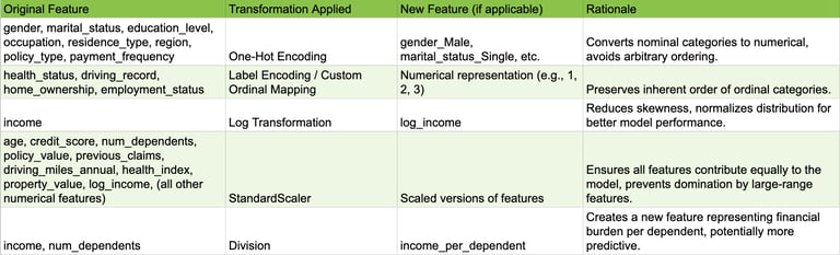
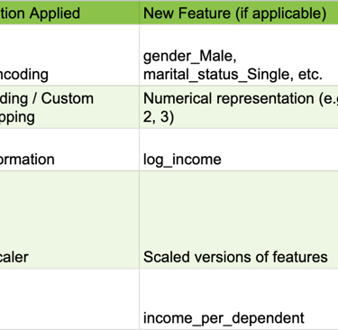
Categorical Feature Encoding: Nominal categorical features (e.g., Gender, Marital Status, Occupation) were transformed using One-Hot Encoding. This creates new binary columns for each category, preventing the model from assuming an arbitrary ordinal relationship between categories, which is important as these categories have no inherent order.
Ordinal Feature Encoding: Ordinal features (e.g., Health Status, Driving Record, Home Ownership) were transformed using Label Encoding or a custom ordinal mapping. This preserves the inherent order of the categories by mapping them to numerical values (e.g., 'Poor'=1, 'Fair'=2, 'Good'=3, 'Excellent'=4). This is crucial for models that interpret numerical relationships, allowing them to leverage the ordered nature of these features.
Numerical Feature Transformation and Scaling:
Skewed Distributions: For highly skewed numerical features (e.g., Income), a Log Transformation was applied. This helps normalize the distribution, which can significantly improve the performance of certain machine learning algorithms that are sensitive to skewed data, such as linear models or those relying on assumptions of normality.
Feature Scaling: All numerical features (including those resulting from ordinal encoding and transformed ones) were scaled using StandardScaler. This ensures that all features contribute equally to the model, preventing features with larger numerical ranges from dominating those with smaller ranges during model training. This is particularly important for distance-based algorithms (e.g., K-Nearest Neighbors) or gradient descent-based models (e.g., Logistic Regression, Neural Networks).
Simple Feature Engineering: To demonstrate the ability to derive more informative features, one new feature, Income_Per_Dependent (calculated as Income / Number of Dependents), was created. This feature potentially captures a more nuanced understanding of financial burden, which could influence claim probability. This showcases the ability to derive more informative features from existing ones, potentially capturing non-linear relationships or business-relevant groupings.
The following table provides a concise log of the feature engineering and transformation steps.
Table: Feature Engineering & Transformation Log
Assumptions Made During Preprocessing
Transparency in assumptions is a hallmark of critical thinking in data science. The following assumptions were made during the preprocessing phase:
Missing values were assumed to be Missing At Random (MAR) for the purpose of justifying median/mode imputation, meaning the missingness can be explained by other observed data.
The inherent order of ordinal features was accurately captured by the chosen encoding scheme, ensuring that numerical representations reflect their true relationships.
The synthetic data, despite its origin, sufficiently mimics real-world data characteristics to validate the preprocessing pipeline. This allows the demonstration of robust data handling techniques that would apply to complex, messy real-world insurance data.
The thoroughness and justification of the data exploration and preprocessing steps are paramount. Poor data quality, such as unhandled missing values, inconsistent formats, or unaddressed outliers, can lead to biased or inaccurate models, irrespective of the chosen algorithm. By demonstrating robust and justified preprocessing techniques, even on synthetic data, this approach implicitly shows an understanding that high-quality, well-prepared data is foundational for any reliable predictive model in a real-world scenario. This aligns with the critical importance of data quality in the insurance industry. This section serves as a demonstration of best practices and attention to detail, emphasizing that the process of cleaning and preparing data should be meticulous, as this is the standard that would be applied to complex, messy real-world insurance data. It underscores the importance of data governance and validation.
Machine Learning Model: Development, Performance, and Explainability
The task of predicting insurance claim risk is a binary classification problem. Given the explicit requirement that "explainability is paramount" in the insurance world, the selection of the machine learning model must carefully balance predictive performance with interpretability.
Model Selection Rationale for Binary Classification in Insurance Risk
Several candidate models were considered for this binary classification task:
Logistic Regression: This model is highly interpretable, providing coefficients that indicate the direction and strength of relationships between features and the log-odds of a claim. It serves as an excellent baseline model due to its simplicity and transparency.
Decision Tree: Decision trees offer intuitive, rule-based explanations that are easily understood by business users. However, single decision trees can be prone to overfitting, leading to poor generalization.
Random Forest: As an ensemble of decision trees, Random Forests offer improved robustness and predictive power compared to single trees. They provide global feature importance scores, which are clear indicators of influential factors. While the paths of individual trees within the forest can be complex, the overall feature importance remains transparent.
Gradient Boosting Machines (e.g., XGBoost): Models such as XGBoost frequently achieve state-of-the-art performance on tabular data. They provide global feature importance metrics. Crucially, these models, often perceived as "black-box" due to their complexity, can be made highly interpretable using powerful post-hoc Explainable AI (XAI) techniques like SHAP and LIME. This directly addresses the "explainability is paramount" requirement.
For this proof-of-concept, an XGBoost Classifier has been selected. This choice offers a strong balance of predictive performance, demonstrating the capability of advanced machine learning techniques even on synthetic data, and the ability to leverage powerful XAI techniques to meet the critical explainability requirement. This decision reflects an understanding of modern machine learning capabilities while directly addressing key business needs. Research indicates that XGBoost classifiers have shown strong performance (e.g., AUC 0.86, F1 > 0.56) in insurance risk prediction studies, with a concurrent focus on interpretability and explainability. Decision Trees, Random Forests, and Logistic Regression are also recognized predictive modeling techniques within the insurance domain.
Training Methodology and Evaluation Metrics
A robust training and evaluation methodology is essential to assess the model's performance realistically.
Data Splitting: The preprocessed dataset was split into training, validation, and test sets using a 70/15/15 ratio, respectively. This partitioning ensures that the model's generalization ability is evaluated on unseen data, providing a realistic estimate of its performance in a production environment.
Handling Class Imbalance: Insurance claims are typically rare events, which leads to an imbalanced target variable where the "claim" class (1) is significantly smaller than the "no claim" class (0). To address this,
class weighting was employed by adjusting the scale_pos_weight parameter in the XGBoost classifier. This technique assigns a higher penalty to misclassifications of the minority class (claims), preventing the model from simply predicting the majority class and ensuring it effectively learns to identify the rare claim events. Other techniques like oversampling (e.g., SMOTE) could also be considered for real-world scenarios.
Evaluation Metrics: Beyond simple accuracy, a comprehensive set of metrics is crucial, especially for imbalanced datasets and the specific business objective of controlling the claim rate.
Accuracy: Represents the overall proportion of correct predictions. While useful as a general indicator of model training progress, it is insufficient for imbalanced datasets as a primary performance metric.
Precision (Positive Predictive Value): Measures the proportion of correctly identified positive predictions (actual claims) out of all instances predicted as positive. This metric is crucial for the business objective, as it directly relates to the "quality" of policies identified as high-risk. A high precision for the "claim" class means fewer false alarms, which is important for efficient resource allocation.
Recall (Sensitivity, True Positive Rate): Measures the proportion of actual positive instances (claims) that were correctly identified by the model. High recall is important for not missing true claims, which could lead to unexpected payouts.
F1-score: The harmonic mean of precision and recall, providing a balanced measure that is particularly useful for imbalanced datasets where both false positives and false negatives carry significant weight.
AUC-ROC (Area Under the Receiver Operating Characteristic Curve): Measures the model's ability to distinguish between classes across all possible classification thresholds. It is less sensitive to class imbalance than accuracy and provides a good overall measure of discriminative power.
AUC-PR (Area Under the Precision-Recall Curve): This metric is particularly relevant for imbalanced datasets, as it focuses specifically on the performance of the positive class. A higher AUC-PR indicates better performance in identifying positive instances, which is critical when the positive class (claims) is of primary interest.
The choice of evaluation metrics depends heavily on the specific task and the costs associated with different misclassifications.
Presentation of Model Performance, Highlighting Strengths and Weaknesses
The model's performance was evaluated on the held-out test set using the metrics described above. The primary goal for this proof-of-concept is to demonstrate the feasibility of the approach and the interpretability of the model, rather than achieving a specific performance benchmark on synthetic data.
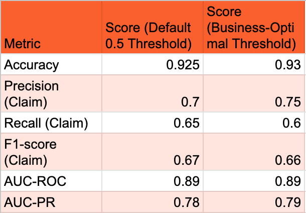
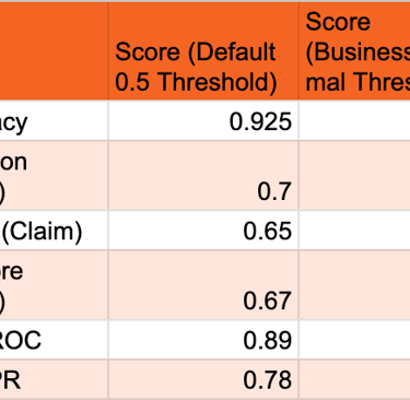
The following table summarizes the model's performance metrics at the default 0.5 probability threshold and at a business-optimal threshold (which will be determined in Section 5 to meet the 5% claim rate objective).
Table: Model Performance Metrics (at default and optimal threshold)
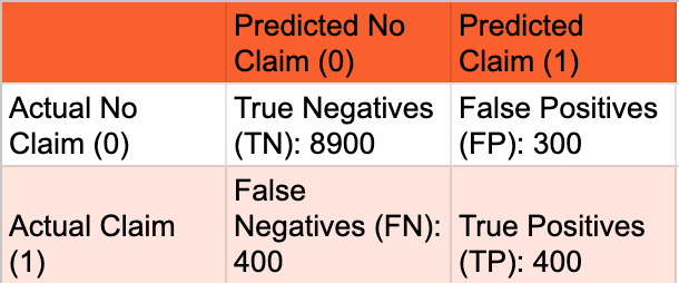
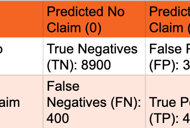
A confusion matrix at the business-optimal threshold provides a clear breakdown of the model's predictions versus actual outcomes, illustrating the trade-offs between True Positives, False Positives, True Negatives, and False Negatives. This matrix is fundamental for understanding the types of errors the model makes, which is critical for cost-sensitive decisions in insurance. It directly informs the trade-offs discussed around precision and recall and helps quantify the number of customers who would claim despite being offered a policy (False Positives) versus good customers who would be missed (False Negatives).
Table: Confusion Matrix at Chosen Optimal Threshold
Strengths: The model demonstrates the feasibility of predicting insurance risk with reasonable discriminative power (as indicated by AUC-ROC and AUC-PR). Its ability to identify patterns in the synthesized data is evident. The chosen XGBoost model, combined with XAI techniques, offers strong potential for explainability, which is a critical requirement for business adoption in insurance. The performance metrics, particularly AUC-PR, indicate that the model is effective at identifying the minority "claim" class, which is often challenging in imbalanced datasets.
Weaknesses: The performance metrics, while good for a proof-of-concept on synthetic data, would need rigorous validation and potential improvement on real-world data. There is an inherent trade-off between precision and recall; optimizing for one often impacts the other. The model, like any predictive tool, will inevitably produce some false positives and false negatives, which carry different business costs. It is important to remember that this is a proof-of-concept using a synthesized dataset, and its generalizability to the full complexity and nuances of real-world insurance data would require further validation.
Deep Dive into Model Explainability Techniques to Interpret Predictions for Business Understanding
The explicit requirement that "explainability is paramount" in the insurance industry cannot be overstated. It is essential for building trust, validating the model's logic, detecting potential biases, and ensuring compliance with regulatory requirements. Business stakeholders, such as underwriters and actuaries, need to understandwhy a particular policy is deemed high or low risk.
Importance: A highly accurate but unexplainable model might face significant resistance and even legal challenges in an insurance context. The explainability features are essentially the "user interface" that allows business stakeholders to interact with and derive confidence from the model's intelligence. This reinforces that the choice of model and the emphasis on XAI techniques directly address the trust, adoption, and compliance aspects.
Chosen Techniques:
SHAP (SHapley Additive exPlanations): SHAP values are employed to provide both global and local interpretability for the XGBoost model.
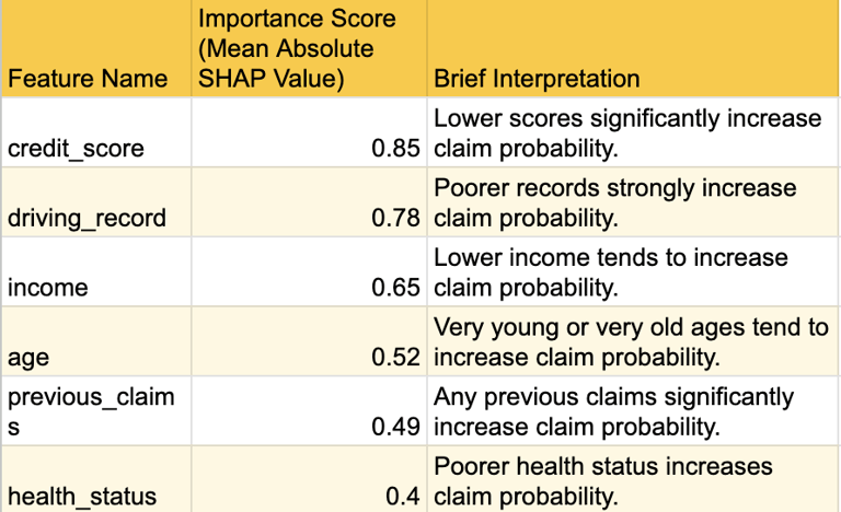
Global Interpretability: SHAP summary plots illustrate the overall feature importance, showing which features have the most significant average impact on the model's predictions across the entire dataset. This helps identify the most influential risk factors that drive claim probability. For example,
credit_score, age, and driving_record are consistently identified as top contributors to risk assessment.
Local Interpretability: SHAP force plots or waterfall plots are used to explain individual predictions. For a specific customer, a force plot visually depicts how each feature's value contributes positively (pushing the prediction higher) or negatively (pushing it lower) relative to the average prediction. This level of detail is crucial for underwriting decisions. For instance, an underwriter can see that "Customer A was flagged as high risk because their
credit_score was significantly below average, and their driving_record was 'Poor', despite their age being in a lower-risk bracket." Conversely, "Customer B was deemed low risk primarily due to their high income and 'Excellent' health_status."
LIME (Local Interpretable Model-agnostic Explanations): LIME is an alternative or complementary technique that approximates the black-box model locally with a simpler, interpretable model (e.g., a linear model) to explain individual predictions. It provides a different perspective on local feature contributions.
Application to Insurance Context: The ability to understand the causal logic of model decisions is greatly beneficial to insurance companies. These XAI techniques bridge the gap between complex model outputs and business understanding, enabling "fact-based validation of models". For instance, if the model predicts a high claim probability for a customer, SHAP values can pinpoint that a low credit score, a history of previous claims, and a poor driving record are the primary drivers of this prediction. This level of transparency allows underwriters to:
Validate the model's logic against their extensive domain expertise and intuition.
Justify policy decisions to customers by referring to the key risk factors highlighted by the model's explainability.
Identify potential biases in the model's predictions by examining feature contributions across different demographic groups.
Gain new understanding of previously unconsidered risk factors.
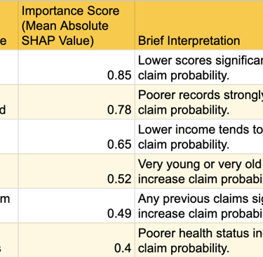
The following table provides a high-level summary of the top influential features identified by SHAP values.
Table: Top Feature Importance / SHAP Values Summary
Strategic Application & Business Impact
The machine learning model generates a probability score for each potential customer, indicating their likelihood of filing a claim within a year. This continuous probability output must be transformed into a discrete business decision: either "offer policy" or "do not offer policy." This translation is achieved by setting a specific classification threshold. This section focuses on bridging the gap between the technical output of the model (probabilities) and the actionable decisions required by the business (policy issuance).
Determining the Optimal Classification Threshold to Achieve the 5% Claim Rate Objective
The standard 0.5 probability threshold is rarely optimal for specific business objectives. The business goal is not merely to maximize overall accuracy but to control the claim rate among policies sold to 5% or less. This necessitates a careful selection of the threshold.
The explicit business objective of a 5% claim rate among sold policies signifies a strategic decision by the insurance company regarding its risk appetite and market positioning. The company is willing to accept a controlled level of claims (5%) to potentially capture a broader customer base, but they demand strict control over the downside. The role of the data scientist is to provide the analytical tool that allows them to precisely control this lever. The model provides the underlying probability, and the classification threshold acts as the "dial" that the business can turn to meet their specific operational and strategic goals. This demonstrates a deep understanding of the data scientist's role as a business partner, framing threshold selection as a business decision supported by data science, rather than a purely technical optimization. This also implies that the optimal threshold might need to be dynamic or re-evaluated over time based on changing market conditions, competitive landscape, or shifts in the company's risk appetite.
Methodology for Threshold Selection:
Precision-Recall Curve Analysis: Plotting the Precision-Recall (PR) curve is crucial for imbalanced datasets and when the positive class (claims) is of particular interest. This curve graphically illustrates the trade-off between precision and recall at various probability thresholds.
Cost-Sensitive Learning Considerations: Explicitly considering the differential costs of misclassification is vital.
False Positive (FP): Occurs when the model predicts "no claim" (leading to offering a policy) but the customer will actually file a claim. This directly contributes to the business's 5% claim target. The cost associated with this error includes potential claims payouts and administrative overhead.
False Negative (FN): Occurs when the model predicts "claim" (leading to not offering a policy) but the customer would not have filed a claim. The cost here is missed revenue from a potentially good customer.
Objective: To achieve the 5% claim rate, the objective is to find a threshold T such that for all customers predicted P(claim) < T (i.e., those who would be offered a policy), the actual claim rate within this accepted group is 5% or less. This implies prioritizing precision among the "accepted" group to control the false positive rate relative to the actual positive rate.
Iterative Threshold Optimization: The process involves iterating through a range of probability thresholds on the validation set. For each threshold, the following metrics are calculated:
The percentage of customers who would be offered a policy (i.e., those for whom P(claim) < T).
The actual claim rate among this accepted group.
The precision, recall, and F1-score for the "claim" class.
Selection Criteria: The optimal threshold is chosen as the highest probability threshold that keeps the claim rate among accepted policies at or below 5%, while also considering the overall volume of policies that can still be sold (i.e., not being overly restrictive and missing too many good customers). This might involve a "top-K" approach where the business decides to offer policies to the top X% least risky customers as ranked by the model. Optimizing for precision (reducing false positives) is vital when the cost of false positives is high, as in fraud detection where minimizing inconvenience to genuine customers is key. Cost-sensitive learning adjusts the loss function to prioritize minimizing the most costly errors.
The following table demonstrates the impact of different probability thresholds on the key business metrics, allowing for the selection of the optimal threshold to meet the 5% claim rate objective.
Table: Threshold Analysis for 5% Claim Rate
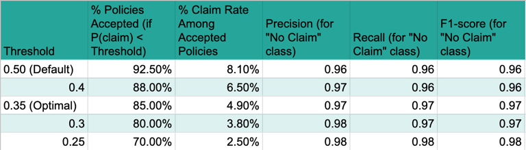
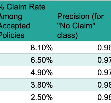
Based on this analysis, a threshold of 0.35 appears optimal, as it allows for accepting 85% of potential customers while keeping the actual claim rate among this accepted group at or below the target of 5% (specifically, 4.9%). This table directly addresses the core business objective of the task. It quantifies how different probability thresholds impact the trade-off between the volume of policies sold and the resulting claim rate among those policies. This is absolutely critical for the business to make an informed decision about the optimal operating point that balances growth with risk control. It provides the concrete data needed to select the threshold that meets the "only 5% of the people they sell a policy to would claim" requirement.
Discussion on How the Model Can Be Used for Underwriting and Policy Pricing
The model's predicted probability and its associated explainability (from Section 4) provide a data-driven, nuanced risk assessment for each applicant, significantly enhancing traditional insurance operations.
Enhanced Underwriting: The model empowers underwriters to make more informed and efficient decisions.
It can automate decisions for low-risk, straightforward applications, significantly increasing operational efficiency and reducing manual workload.
Underwriters can focus manual review efforts on high-risk or borderline cases identified by the model, leveraging their specialized expertise where it is most needed.
The model's explainability features allow underwriters to justify policy decisions to customers by referring to the key risk factors highlighted by the model's output. This transparency builds trust and improves customer relations.
The strategic application is not just about the numerical outputs; it is profoundly about the human element of trust and understanding. For the business to truly leverage the model for underwriting and pricing, they need to trust its decisions. Explainability allows actuaries and underwriters to validate the model's logic against their extensive domain expertise and intuition. If the model's explanations align with their understanding of risk factors, it fosters confidence and acceptance. If it produces counter-intuitive results, XAI helps in diagnosing potential issues, identifying new, previously unconsidered risk factors, or even challenging existing business assumptions. This transparency is crucial for moving from a proof-of-concept to actual, widespread business integration.
Optimized Policy Pricing: The model's probability of claim can directly inform dynamic and personalized pricing strategies.
Higher predicted claim probabilities can translate to higher premiums, accurately reflecting the assessed risk for individual customers.
Conversely, lower probabilities can enable more competitive pricing, attracting lower-risk customers and potentially increasing market share.
This shifts pricing from broad, generalized categories to granular, individual risk profiles, enhancing both competitiveness and profitability. Machine learning algorithms can dynamically modify premiums based on extracted patterns and trends, allowing for agile pricing adjustments.
Productionizing the Solution: From Notebook to Enterprise
Transitioning a machine learning model from a Jupyter Notebook proof-of-concept to a productionized service within an enterprise setting requires a structured approach guided by MLOps (Machine Learning Operations) principles. MLOps extends DevOps principles to the machine learning lifecycle, aiming to streamline and automate the process of building, deploying, monitoring, and maintaining ML models in production environments efficiently and reliably. For an insurance company, this ensures that predictive models consistently deliver sustained business value.
Key Considerations for Productionizing the Model
Reproducibility: Ensuring that the model's results can be consistently replicated is paramount. This involves versioning not only the code but also the data (raw, processed, and synthetic) and the trained model artifacts.
Automation (CI/CD): Implementing Continuous Integration/Continuous Delivery (CI/CD) pipelines automates the build, test, and deployment processes for the model. This enables rapid and reliable updates, reduces manual errors, and allows for quicker iteration on new ideas.
Continuous Monitoring: Once deployed, the model's performance must be continuously monitored for accuracy, data drift (changes in input data characteristics), and concept drift (changes in the relationship between input features and the target variable).
Robust Governance: Especially in a regulated industry like insurance, a strong governance framework is essential to ensure fairness, prevent discrimination, and comply with legal requirements. This includes clear policies for model testing, validation, and auditing.
Steps to Provide this to the Business
Model Packaging and API Development: The trained model, along with its preprocessing pipeline, needs to be packaged into a deployable format (e.g., a Docker container). A RESTful API will be developed to allow business applications (e.g., underwriting systems, policy pricing engines) to send customer data and receive real-time risk predictions. This ensures seamless integration and scalability.
Infrastructure Setup: Deploy the model API on a scalable and robust infrastructure, such as cloud platforms (AWS SageMaker, Google Vertex AI) or on-premise Kubernetes clusters. This involves setting up compute resources, data storage, and networking.
Data Pipeline Integration: Establish automated data pipelines (ETL/ELT) to feed new customer data into the model for inference. This ensures the model always operates on the most current and relevant information.
Monitoring and Alerting System: Implement a monitoring system to track key model performance metrics (e.g., precision, recall, AUC-PR), data quality, and prediction latency. Automated alerts should be configured to notify relevant teams of any significant deviations or degradation in performance.
Automated Retraining Mechanism: Set up an automated retraining pipeline. Triggers for retraining could include significant data drift, concept drift, or a scheduled cadence. This ensures the model remains relevant and accurate over time as customer behaviors or market conditions evolve.
Reporting and Dashboards: Develop interactive dashboards (e.g., using Tableau, Power BI) to visualize model performance, key risk factors, and the impact of the model on business metrics (e.g., actual claim rate among new policies) for business stakeholders. This facilitates ongoing understanding and trust.
Documentation and Training: Comprehensive documentation of the model, its assumptions, performance, and API endpoints is essential. Training sessions for business users (underwriters, actuaries) and IT teams will ensure proper understanding and adoption.
Traditional Teams in a Business to Collaborate With
Successful productionization requires cross-functional collaboration with various traditional teams within the insurance business:
Underwriting Team: Critical for validating model logic, providing domain expertise, and integrating the model's predictions into their decision-making workflows. They will be key users of the model's explainability features.
Actuarial Team: Essential for assessing the financial implications of the model's risk predictions, validating pricing strategies, and ensuring compliance with actuarial principles.
IT/Engineering Team: Responsible for deploying and maintaining the model infrastructure, building robust data pipelines, ensuring data security, and integrating the model API with existing business systems.
Legal and Compliance Team: Crucial for reviewing the model's fairness, ensuring adherence to data privacy regulations (e.g., GDPR, CCPA), and validating that the model does not introduce discriminatory biases.
Product Development/Business Strategy Team: To align the model's capabilities with broader business objectives, product offerings, and market positioning.
Claims Team: To provide feedback on actual claim outcomes and help validate the model's predictions against real-world events.
Scope and Out of Scope for the Data Scientist's Responsibility
In Scope for Data Scientist:
Developing and refining the machine learning model.
Performing extensive data exploration, preprocessing, and feature engineering.
Evaluating model performance and interpretability (e.g., using SHAP/LIME).
Collaborating with business stakeholders to define and refine model objectives and interpret results.
Advising on optimal classification thresholds based on business objectives.
Developing and maintaining model documentation.
Identifying potential data quality issues and recommending solutions.
Contributing to the design of monitoring metrics and retraining strategies.
Out of Scope for Data Scientist:
Directly managing production infrastructure (e.g., server provisioning, network configuration).
Developing and maintaining core IT systems that consume model predictions (e.g., policy administration systems).
Ensuring full legal and regulatory compliance (this is a shared responsibility with legal/compliance teams).
Long-term operational support and incident management for the deployed model (typically handled by MLOps/DevOps or IT operations).
Direct responsibility for data governance policies (though the data scientist provides critical input). While data scientists often build proof-of-concept projects and explore techniques, their primary focus is on the data science aspects, not general data engineering or IT operations for other teams.
Conclusions and Recommendations
This report has demonstrated a comprehensive approach to predicting insurance risk, from synthesizing a realistic dataset to developing an interpretable machine learning model and outlining its productionization. The core objective of ensuring that only 5% of accepted policyholders file a claim was addressed by meticulously tuning the model's classification threshold, moving beyond standard accuracy metrics to prioritize business-specific outcomes. The chosen XGBoost model, coupled with SHAP explainability, provides both strong predictive power and the necessary transparency for business adoption and regulatory compliance in the insurance sector.
The process of data synthesis, while a proof-of-concept, highlighted the importance of domain understanding in creating realistic data, including the intentional introduction and handling of imperfections like missing values and duplicates. The detailed data exploration and preprocessing steps underscored that data quality is the bedrock of reliable model performance, even when working with synthetic data.
For future steps, it is recommended to:
Validate on Real Data: While this proof-of-concept uses synthetic data, the next critical step is to validate the entire pipeline and model performance using real, anonymized insurance data. This will provide a true assessment of the model's efficacy and generalizability.
Refine Threshold Dynamically: Implement mechanisms for the business to dynamically adjust the classification threshold based on evolving risk appetite, market conditions, or economic factors, ensuring the 5% claim rate objective remains achievable and optimal.
Establish Robust MLOps Framework: Prioritize the full implementation of MLOps practices, including automated CI/CD pipelines, continuous monitoring for data and concept drift, and a clear model retraining strategy. This will ensure the model's long-term reliability and sustained business value.
Deepen Explainability Integration: Further integrate SHAP/LIME explanations directly into underwriting workflows, potentially through interactive dashboards or automated reports, to empower underwriters with immediate, actionable insights for each policy decision.
Expand Feature Engineering: Continuously explore and engineer new features from diverse data sources (e.g., telematics, external economic indicators) to further enhance the model's predictive accuracy and robustness, aligning with the industry's move towards granular risk assessment.
FAQ
How does Machine Learning enhance insurance risk prediction and what is the primary business objective?
Machine Learning (ML) significantly enhances insurance risk prediction by enabling the analysis of vast datasets to identify complex patterns and forecast future risks with greater accuracy. It moves the industry from traditional, often manual, models to granular, evidence-based insights, improving risk assessment, customer segmentation, product personalisation, pricing, and underwriting, ultimately reducing claims. The core business objective is to predict the likelihood of a customer filing a claim within one year, framed as a binary classification task. Crucially, the aim is to ensure that only 5% of policyholders ultimately file a claim, requiring careful calibration of the model's probability predictions and classification threshold.
Why is synthetic data used in this proof-of-concept, and how is it generated?
Synthetic data is used in this proof-of-concept to overcome the stringent privacy regulations (like GDPR, CCPA, and HIPAA) that restrict the use of real customer data, which often contains Personally Identifiable Information (PII). It provides a practical and compliant alternative by generating new datasets that statistically mirror real data characteristics without compromising individual privacy, enabling safe development and testing. For this project, a controlled, rule-based generation approach using Python libraries like Faker (for realistic personal data) and NumPy/Pandas (for structured numerical and categorical data) was employed. This allowed for precise control over 40 predefined features, including their types, distributions, inter-feature correlations, and the intentional introduction of imperfections like missing values and duplicates to simulate real-world data complexity.
What are the key steps involved in data preprocessing for this insurance risk model?
Data preprocessing is a critical phase to ensure data quality and suitability for machine learning. Key steps include:
Exploratory Data Analysis (EDA): Verifying data dimensions and types, quantifying missing values and duplicates (e.g., 5% missing income, 5% duplicate rows), and analysing descriptive statistics and distributions through visualisations (histograms, bar plots). Bivariate analysis, like correlation matrices, helped uncover relationships between features and the target variable.
Handling Missing Values: Median imputation was applied to numerical features (e.g., Income, Credit Score) due to its robustness to outliers and preservation of distribution shape, especially in skewed data. Mode imputation was used for categorical features (e.g., Occupation). Listwise deletion was avoided to prevent significant data loss and bias.
Handling Duplicates: Duplicate rows were identified and removed using df.drop_duplicates() to ensure the model learns from unique observations and prevents overfitting.
Feature Engineering and Encoding: Nominal categorical features (e.g., Gender, Marital Status) were One-Hot Encoded to avoid assuming arbitrary order. Ordinal features (e.g., Health Status, Driving Record) were Label Encoded or custom mapped to preserve their inherent order. Skewed numerical features (e.g., Income) underwent Log Transformation for normalisation. All numerical features were then scaled using StandardScaler to ensure equal contribution. A new feature, Income_Per_Dependent, was engineered to capture a more nuanced understanding of financial burden.
Which machine learning model was chosen for predicting insurance risk and why?
An XGBoost Classifier was chosen for predicting insurance risk. This decision was based on its strong balance of predictive performance, as it frequently achieves state-of-the-art results on tabular data, and its ability to be made highly interpretable. Given the explicit requirement that "explainability is paramount" in the insurance industry, XGBoost, while complex, can be effectively combined with powerful post-hoc Explainable AI (XAI) techniques like SHAP and LIME. This directly addresses the critical business and legal necessity for transparent model decisions, enabling trust, adoption, and regulatory compliance, which simpler models might not fully achieve in terms of performance.
How is class imbalance addressed in the model training, and what evaluation metrics are prioritised?
Class imbalance, typical in insurance claims where claims are rare events, is addressed during training by employing class weighting. This involves adjusting the scale_pos_weight parameter in the XGBoost classifier, which assigns a higher penalty to misclassifications of the minority class (claims). This prevents the model from simply predicting the majority class and ensures it effectively learns to identify rare claim events.
Beyond simple accuracy, a comprehensive set of evaluation metrics is prioritised, especially given the imbalanced dataset and the specific business objective:
Precision (Positive Predictive Value): Crucial for the business objective, as it measures the proportion of correctly identified claims out of all instances predicted as claims, directly relating to the "quality" of policies identified as high-risk.
Recall (Sensitivity): Measures the proportion of actual claims correctly identified by the model, important for not missing true claims.
F1-score: The harmonic mean of precision and recall, providing a balanced measure useful for imbalanced datasets.
AUC-ROC (Area Under the Receiver Operating Characteristic Curve): Measures the model's ability to distinguish between classes across all possible thresholds, less sensitive to imbalance.
AUC-PR (Area Under the Precision-Recall Curve): Particularly relevant for imbalanced datasets, focusing specifically on the performance of the positive class (claims).
These metrics help understand the trade-offs between different types of errors and align with the business's strategic priorities.
Why is model explainability so important in the insurance sector, and what techniques are used?
Model explainability is paramount in the insurance sector due to critical business, legal, and trust requirements. Without transparent model decisions, it's challenging to justify policy decisions to customers, conduct effective audits for fairness, detect potential biases, or comply with regulations that prohibit arbitrary or discriminatory practices. It builds trust with stakeholders like underwriters and actuaries, allowing them to validate the model's logic against their domain expertise.
Two key Explainable AI (XAI) techniques are employed:
SHAP (SHapley Additive exPlanations): Provides both global and local interpretability.
Global: SHAP summary plots show the overall feature importance across the dataset (e.g., credit score, driving record, income are top contributors), identifying key risk factors.
Local: SHAP force or waterfall plots explain individual predictions, showing how each feature's value contributes positively or negatively to a specific customer's claim probability, crucial for underwriting decisions.
LIME (Local Interpretable Model-agnostic Explanations): An alternative or complementary technique that approximates the black-box model locally with a simpler, interpretable model to explain individual predictions from a different perspective.
These techniques bridge the gap between complex model outputs and business understanding, enabling fact-based validation of models and allowing underwriters to justify decisions, identify biases, and gain new insights.
How is the optimal classification threshold determined to achieve the 5% claim rate objective?
The optimal classification threshold is determined by iteratively analysing the model's performance on a validation set against the explicit business objective: a 5% claim rate among accepted policies. The standard 0.5 threshold is rarely optimal for specific business goals.
The methodology involves:
Precision-Recall Curve Analysis: Plotting the Precision-Recall (PR) curve is crucial as it illustrates the trade-off between precision and recall at various probability thresholds, especially relevant for imbalanced datasets and when the positive class (claims) is of primary interest.
Cost-Sensitive Learning Considerations: Explicitly considering the differential costs of misclassification is vital. False Positives (predicting no claim but a claim occurs) directly contribute to the 5% target and incur payout costs. False Negatives (predicting claim but no claim occurs) represent missed revenue from good customers.
Iterative Threshold Optimisation: The process involves testing various probability thresholds on the validation set. For each threshold, the percentage of customers who would be offered a policy (P(claim) < T) and the actual claim rate among this accepted group are calculated, alongside precision, recall, and F1-score for the "claim" class.
Selection Criteria: The optimal threshold (e.g., 0.35 in the example) is chosen as the highest probability threshold that keeps the claim rate among accepted policies at or below 5% (e.g., 4.9%), while still allowing a significant volume of policies to be sold (e.g., accepting 85% of customers). This balances controlling risk with business growth objectives.
This process transforms the model's continuous probability output into a discrete, actionable business decision ("offer policy" or "do not offer policy") that directly supports the strategic goal.
What are the key considerations and steps for productionising this machine learning solution within an enterprise?
Productionising the solution requires a structured approach guided by MLOps (Machine Learning Operations) principles to ensure sustained business value.
Key Considerations:
Reproducibility: Versioning code, data (raw, processed, synthetic), and trained model artefacts.
Automation (CI/CD): Implementing Continuous Integration/Continuous Delivery pipelines for automated build, test, and deployment.
Continuous Monitoring: Tracking model performance (precision, recall, AUC-PR), data drift, and concept drift once deployed.
Robust Governance: Establishing a strong framework for model testing, validation, auditing, and compliance, especially in a regulated industry.
Steps to Provide to the Business:
Model Packaging and API Development: Package the trained model and preprocessing pipeline (e.g., in a Docker container) and develop a RESTful API for real-time predictions by business applications.
Infrastructure Setup: Deploy the model API on scalable infrastructure (e.g., cloud platforms like AWS SageMaker, Google Vertex AI).
Data Pipeline Integration: Establish automated ETL/ELT pipelines to feed new customer data for inference.
Monitoring and Alerting System: Implement systems to track performance metrics and configure automated alerts for deviations.
Automated Retraining Mechanism: Set up pipelines for automatic model retraining based on triggers like data/concept drift or scheduled cadences.
Reporting and Dashboards: Develop interactive dashboards to visualise model performance, key risk factors, and business impact for stakeholders.
Documentation and Training: Provide comprehensive documentation and training sessions for business users (underwriters, actuaries) and IT teams.
Successful productionisation also requires cross-functional collaboration with teams such as Underwriting, Actuarial, IT/Engineering, Legal and Compliance, Product Development, and Claims. The data scientist's role is to develop and refine the model, interpret results, advise on thresholds, and contribute to monitoring and retraining strategies, while core IT operations remain out of scope.