Understanding Fact and Dimension Tables in Data Warehousing

This report provides a comprehensive examination of the principles and practices of dimensional modeling, the predominant paradigm for designing enterprise data warehouses. It deconstructs the foundational components—fact tables, which store quantitative business measurements, and dimension tables, which provide descriptive context. The analysis extends to the architectural schemas (Star and Snowflake) that structure their relationship, the typologies of both table types, and the critical techniques for managing temporal data, such as Slowly Changing Dimensions (SCDs). By synthesizing foundational theory with practical application, this document elucidates how the dimensional model serves as a high-performance and business-intuitive foundation for modern business intelligence and analytics.

The Foundational Dichotomy of Dimensional Modeling

The architecture of modern data warehousing is built upon a foundational principle: the deliberate and strategic separation of data into two distinct and complementary categories. On one side are the quantitative, numeric measurements of business processes, known as facts. On the other is the qualitative, descriptive context that gives meaning to these measurements, known as dimensions. This fundamental dichotomy is the cornerstone of dimensional modeling, an approach designed to construct data warehouses that are simultaneously optimized for high-performance querying and are intuitively understandable to business users.

Dimensional modeling was developed not as a mere technical preference but as a strategic solution to bridge the profound gap between two different data paradigms. Transactional systems, designed for Online Transaction Processing (OLTP), are typically normalized to ensure data integrity and efficiency for day-to-day operations like inserting, updating, and deleting small records. However, this normalization scatters business information across a complex web of tables, rendering it ill-suited for the demands of Online Analytical Processing (OLAP), which involves complex queries across large historical datasets. The dimensional model addresses this challenge by reorganizing data specifically for analytical inquiry.

The entire discipline of dimensional modeling can be understood as a sophisticated exercise in balancing a critical set of trade-offs. Designers must constantly weigh the need for raw query performance against the imperative of data integrity, the benefits of storage efficiency against the demand for ease of use, and the elegance of structural simplicity against the necessity of analytical flexibility. The enduring success of this model stems from its structural alignment with the cognitive patterns of business inquiry. Business users do not think in terms of third normal form; they ask questions like, "Show me the total sales (a fact) for the electronics category (a dimension attribute) in the last quarter (another dimension attribute)". The dimensional model physically organizes data to mirror this natural pattern of questioning, placing a central table of metrics (facts) in direct relationship with surrounding tables of context (dimensions). It is this inherent "business friendliness" that lowers the barrier to self-service analytics and makes data accessible to the decision-makers who depend on it.

The Anatomy of a Fact Table: The Quantitative Core

At the gravitational center of every dimensional model lies the fact table. It is the repository for the fundamental measurements of the enterprise and the ultimate target of the vast majority of data warehouse queries. This chapter deconstructs the purpose, structure, and typologies of fact tables, establishing their role as the quantitative heart of the analytical system.

1.1 Defining the Fact Table: Purpose and Structure

The primary purpose of a fact table is to store the quantitative essence of business events—the measurements, metrics, or "facts" associated with a specific business process. These numeric values, such as

SalesAmount, UnitsSold, or TransactionCount, represent the performance and operational outcomes that an organization seeks to analyze.

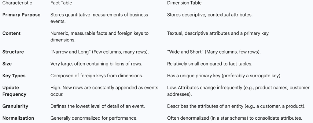
Structurally, fact tables are characterized as being "narrow and long" or "deep." They typically have a relatively small number of columns but can grow to contain billions or even trillions of rows, as each row corresponds to a specific event that has occurred over time. The columns within a fact table are of two principal types:

1. Numeric Measures: These are the facts themselves, the quantitative data that will be aggregated and analyzed.

2. Foreign Keys: These columns serve as connectors, linking each row in the fact table to the corresponding descriptive records in the various dimension tables (e.g., ProductKey, DateKey, CustomerKey).

In addition to these, a fact table may also contain specialized attributes like degenerate dimensions or audit columns that track data lineage and ETL processes.

1.2 Key Characteristics of Fact Tables

Two characteristics are paramount in the design of a robust fact table: its grain and the additivity of its measures.

1.2.1 Granularity

Granularity is the single most important concept in dimensional design. It defines precisely what a single row in a fact table represents. The declaration of the grain—for example, "one row per individual line item on a sales receipt" or "one row per student per class attended per day"—is the foundational step upon which the entire model is built. An unambiguous grain ensures that all measures stored in the fact table are consistent and that queries produce accurate, predictable results.

1.2.2 Additivity of Measures

The analytical utility of a measure is determined by its additivity—the extent to which it can be summed across dimensions. Measures fall into three distinct categories:

• Additive: These are the most flexible and desirable measures. They can be meaningfully summed across all associated dimensions. SalesQuantity and Revenue are classic examples; one can sum sales quantity across all products, all stores, and all time periods.

• Semi-Additive: These measures can be summed across some dimensions but not others. The most common example is a balance or inventory level. An inventory count can be summed across different products or warehouses to get a total inventory level at a specific point in time, but it cannot be summed across the time dimension (e.g., adding Monday's inventory to Tuesday's inventory is a meaningless calculation).

• Non-Additive: These measures cannot be meaningfully summed across any dimension. Ratios, percentages, and temperatures are common examples. A ProfitMargin percentage, for instance, cannot be directly summed. To correctly aggregate non-additive measures, their component parts (e.g., Profit and Revenue) must be stored as additive facts in the table. The non-additive ratio can then be calculated from the summed components at query time.

1.3 A Deep Dive into Fact Table Typologies

The business process being modeled dictates the appropriate type of fact table to use. The three fundamental types—transactional, periodic snapshot, and accumulating snapshot—are not interchangeable; each is designed to answer a different class of business questions.

1.3.1 Transactional Fact Tables

The transactional fact table is the most common and fundamental type, often serving as the workhorse of the data warehouse. Each row in this table corresponds to a single, discrete event or transaction, captured at its most atomic level of detail, or grain. These tables are characterized by being append-only; new rows are continuously inserted as events occur, but existing rows are never updated. They are ideal for analyzing the intensity of a business process, answering "how many?" or "how much?" questions with high precision.

• Use Case: A retail sales system would use a transactional fact table to record every single item sold in every transaction. Other examples include tracking individual website clicks, phone calls, or financial trades.

1.3.2 Periodic Snapshot Fact Tables

These tables capture the state of a business process at regular, predictable intervals, such as the end of each day, week, or month. Rather than recording every transaction that led to a certain state, a periodic snapshot table provides a summary of performance over that period. Each row represents a "snapshot" in time. These tables are excellent for trend analysis, as they provide a consistent series of measurements over time. They are characterized by semi-additive measures, such as account balances or inventory levels, and are loaded on a regular, scheduled basis.

• Use Case: A bank would use a periodic snapshot to record the closing balance of every customer account at the end of each business day. This allows for analysis of balance trends without needing to process every debit and credit transaction.

1.3.3 Accumulating Snapshot Fact Tables

These tables are designed to track the lifecycle of a process that has a well-defined beginning, middle, and end, composed of multiple, predictable milestones. A single row is created when the process begins and is subsequently updated as each key milestone is reached. This update behavior is unique among fact table types. The table structure is characterized by multiple date foreign keys, one for each milestone (e.g.,

OrderDateKey, ShipDateKey, DeliveryDateKey), which allows for the analysis of the duration, or lag, between stages.

• Use Case: An order fulfillment pipeline is a classic example. A single row would track an order from the moment it is placed, through manufacturing, shipping, and final delivery, with the dates for each stage being updated in the same row. This allows for direct measurement of process efficiency, such as the average time from order to shipment.

1.3.4 Specialized Fact Table Types

Beyond the three fundamental types, several specialized patterns address specific modeling challenges:

• Factless Fact Tables: As the name suggests, these tables contain no numeric measures. Their purpose is to record the occurrence of an event or to model a many-to-many relationship between dimensions. The "fact" is the event itself, which is analyzed by counting the rows in the table that meet certain dimensional criteria.

  • Use Case: Tracking which students attended which classes on which days. There is no numeric measure, but by counting rows, an analyst can determine class attendance rates.

• Aggregate Fact Tables: Also known as summary tables, these are not a fundamental type but rather a performance optimization technique. They contain pre-calculated summaries of data from a more granular base fact table. By storing these aggregates, they can dramatically accelerate queries for high-level reports and dashboards.

  • Use Case: Creating a monthly regional sales summary table from a daily transaction-level sales fact table to speed up performance for an executive dashboard that only displays monthly trends.

The historical reliance on aggregate tables was a direct consequence of hardware limitations, where querying massive transactional tables was computationally prohibitive. However, the advent of modern Massively Parallel Processing (MPP) columnar data warehouses has significantly altered this dynamic. These platforms are so powerful that they can often aggregate billions of rows of raw transaction data on the fly, fast enough for many analytical needs. This technological shift has led to a change in best practices. The high cost of data engineering talent now often outweighs the cost of compute and storage. Consequently, the modern approach frequently favors a "just-in-time" modeling strategy, where teams rely on the raw power of their warehouse and only create aggregate tables when a clear and persistent performance bottleneck is identified, prioritizing engineering flexibility over premature computational optimization.

Table 1: A Guide to Fact Table Types

Fact Table TypeGrainMeasuresUpdate MethodKey CharacteristicsTypical Business QuestionTransactionalOne row per discrete event (atomic level)Fully AdditiveAppend-Only (Insert)Most granular; grows very rapidly.How many units of Product X were sold last week?Periodic SnapshotOne row per entity per defined time periodSemi-AdditiveAppend-Only (Insert)Summarizes status at regular intervals; good for trend analysis.What was the total inventory level for each store at the end of each month?Accumulating SnapshotOne row per process lifecycleAdditive & Semi-Additive (Durations)Insert then UpdateMultiple date keys for milestones; tracks process efficiency.What is the average time from order placement to shipment?

The Anatomy of a Dimension Table: Providing the Contextual Narrative

While fact tables provide the quantitative "what," dimension tables provide the rich, descriptive "who, what, where, when, and why" that makes the data meaningful and analyzable. They are the soul of the data warehouse, transforming raw numbers into business insights. The quality and depth of the dimension tables are often the most significant determinant of a data warehouse's analytical power.

2.1 Defining the Dimension Table: The "Who, What, Where, When, Why"

The purpose of a dimension table is to store the descriptive attributes that are used to filter, group, and label the facts in a query. These attributes are the textual context surrounding a business event, such as product names, customer demographics, geographic locations, and fiscal calendar details.

Structurally, dimension tables are the inverse of fact tables: they are typically "wide and short." They are characterized by having a large number of columns (attributes) but a relatively small number of rows compared to their associated fact tables. For example, a company might have billions of sales transactions but only a few thousand products or a few hundred stores. To enhance ease of use and query performance, dimension tables are often denormalized, meaning that related attributes are grouped together in a single flat table to avoid the need for additional joins during a query. A Product dimension, for instance, would contain not just the product name but also its category, subcategory, brand, and other relevant descriptors in a single record.

2.2 Keys in Dimension Tables: Surrogate vs. Natural Keys

The connection between fact and dimension tables is managed through keys. A critical design choice is the type of primary key used in the dimension table.

• Natural Key: This is the primary key or unique identifier for an entity as it exists in the source operational system, such as an EmployeeID, a ProductSKU, or a government-issued ID number.

• Surrogate Key: This is a system-generated integer primary key that is unique to the data warehouse and has no intrinsic business meaning. It is simply a sequential number (1, 2, 3,...).

The use of surrogate keys as the primary key for dimension tables is a foundational best practice in dimensional modeling. This approach provides several crucial advantages. First, it insulates the data warehouse from changes in the source systems. If a company reorganizes and reassigns all its employee IDs (the natural keys), a data warehouse built on surrogate keys remains unaffected. Second, surrogate keys allow for the seamless integration of data from multiple source systems, where natural keys may overlap or have different formats. Most importantly, they are essential for properly implementing most methods of tracking historical changes in dimensional attributes, a concept known as Slowly Changing Dimensions (SCDs), particularly the vital Type 2 method.

2.3 The Importance of High-Quality Attributes

The analytical power of a dimensional model is a direct function of the quality, depth, and clarity of its dimensional attributes. A "robust" dimension is one that is populated with numerous, well-defined, business-friendly attributes that anticipate the ways in which users will want to analyze the data. This includes establishing clear hierarchies within the dimension, such as

Product -> Subcategory -> Category -> Department or Store -> City -> State -> Country. These hierarchies are not merely descriptive; they are functional, enabling powerful drill-down and roll-up analysis in business intelligence (BI) tools, allowing a user to seamlessly navigate from a high-level summary (e.g., sales by country) to a granular view (e.g., sales by store).

Table 2: Comparative Analysis of Fact and Dimension Tables

The Star and Snowflake Schemas: Architecting the Relationship

The way fact and dimension tables are interconnected defines the schema of the data warehouse. The two predominant architectural patterns are the star schema and the snowflake schema. They represent different philosophical approaches to the fundamental trade-off between query performance and data normalization.

3.1 The Star Schema: Optimized for Simplicity and Performance

The star schema is the simplest and most common dimensional modeling structure. It consists of a central fact table directly connected to a single layer of surrounding dimension tables. When visualized, this structure resembles a star, with the fact table at the center and the dimensions radiating outwards as points.

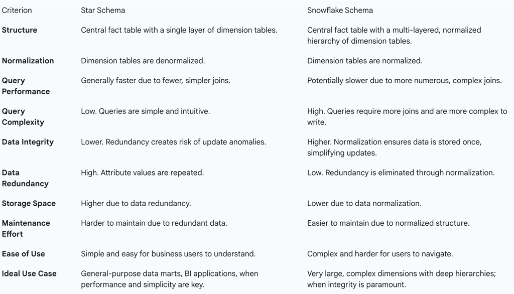
The design philosophy of the star schema prioritizes query performance and ease of use above all else. This is achieved by heavily denormalizing the dimension tables. All attributes related to a given dimension (e.g., product name, category, brand, supplier) are stored in a single, wide dimension table. This design minimizes the number of joins required to answer a business query; typically, a query will join the large fact table to one or more small dimension tables, a pattern that many database engines are specifically optimized to handle (known as a "star join").

• Advantages: The primary benefits are simplicity and speed. The structure is intuitive for business users to understand and for analysts to write queries against. The reduced join complexity leads to significantly faster query performance, and the schema is well-supported by virtually all BI tools, which are often designed with the star schema in mind.

• Disadvantages: The main drawback is data redundancy. Because the dimensions are denormalized, attribute values (like a category name) are repeated for every member of that category. This increases storage requirements and introduces a risk to data integrity; if a category name needs to be updated, it must be changed in many rows, creating the potential for update anomalies. Star schemas are also less adept at handling complex, multi-level hierarchies or many-to-many relationships.

3.2 The Snowflake Schema: Optimized for Normalization and Integrity

The snowflake schema is a logical extension of the star schema. In this model, the denormalized dimension tables are normalized by breaking them down into multiple, related tables. Hierarchical relationships, such as

City -> State -> Country or Product -> Brand -> Manufacturer, are stored in separate tables linked by foreign keys. This creates a more complex, branching structure that resembles the intricate pattern of a snowflake.

The design philosophy of the snowflake schema prioritizes data integrity and storage efficiency. By normalizing the dimensions, it eliminates data redundancy. Each unique attribute value (e.g., a country name) is stored only once in its own table, which reduces the overall storage footprint and makes data maintenance simpler and more reliable. An update to a country name, for example, needs to be made in only one place.

• Advantages: The key benefits are reduced storage space and higher data integrity. The normalized structure is easier to maintain and less prone to update anomalies. It also provides a more robust framework for modeling complex, multi-level dimensional hierarchies.

• Disadvantages: The primary trade-off is complexity. The schema is more difficult for users to understand and requires more complex queries with a greater number of joins to retrieve data. These additional joins can lead to slower query performance compared to the simpler star schema.

3.3 Comparative Analysis and Practical Guidance

The choice between a star and snowflake schema is not about which is universally superior, but which is more appropriate for a specific set of requirements and constraints.

• When to Choose a Star Schema: A star schema is the preferred choice when query performance, simplicity, and speed of development are the primary objectives. It is ideal for data marts focused on a specific subject area and for feeding BI tools that perform best with simple, flat structures. It is the default and most common choice in modern data warehousing.

• When to Choose a Snowflake Schema: A snowflake schema should be considered when data integrity, storage efficiency, and ease of maintenance are critical priorities. It is particularly suitable for modeling very large, complex dimension tables with many levels of hierarchy or for dimensions where attributes are volatile and updated frequently.

Historically, the debate between these two schemas was more pronounced. Snowflake's advantage in saving storage was significant when disk space was expensive. However, the dramatic and ongoing decrease in storage costs has largely negated this benefit, leading to a strong industry preference for the simplicity and performance of the star schema. Concurrently, modern query engines and BI platforms have become more sophisticated, with improved optimizers that can mitigate some of the performance penalty associated with the more complex joins of a snowflake schema.

This technological evolution suggests that the optimal design is often not a pure implementation of one schema or the other, but a pragmatic hybrid. A data architect might adopt the star schema as the default pattern for its simplicity and performance, but selectively "snowflake" a particularly large, complex, or volatile dimension—such as a multi-level product hierarchy or a customer dimension with numerous historical addresses—to gain the maintenance and integrity benefits where they are most impactful, without complicating the rest of the model. The modern best practice is one of selective, justified normalization rather than rigid adherence to a single schema type.

Table 3: Star Schema vs. Snowflake Schema - A Detailed Comparison

Advanced Dimensional Concepts: Specialized Dimensions and Design Patterns

Beyond the basic structures of fact and dimension tables, a set of advanced design patterns has been developed to address common and often complex modeling challenges. These patterns provide elegant solutions for integrating data across the enterprise, managing shared dimensions, and handling miscellaneous attributes.

4.1 Conformed Dimensions

A conformed dimension is a dimension that is shared across multiple fact tables, and often across different data marts, with a consistent structure, content, and meaning. For example, a single, master

Date dimension should be used to analyze sales facts, inventory facts, and marketing facts. Similarly, a Product dimension should be identical whether it is providing context for sales transactions or supply chain movements.

Conformed dimensions are the cornerstone of an integrated enterprise data warehouse. They create a "single version of the truth" for key business entities, ensuring that data can be compared and analyzed consistently across different business processes. This enables powerful cross-functional analysis, such as comparing sales figures with marketing campaign data using the same

Product and Date dimensions, which would be impossible if each data mart had its own unique version of these dimensions.

4.2 Role-Playing Dimensions

A role-playing dimension occurs when a single physical dimension table is referenced multiple times within the same fact table, with each reference representing a distinct role in the business event. The most common example involves the

Date dimension. A single fact table row for an order might need to record the date the order was placed, the date it was shipped, and the date it was delivered. Instead of creating three separate and identical date tables, a single Date dimension is used, and the fact table includes three distinct foreign keys: OrderDateKey, ShipDateKey, and DeliveryDateKey. Each of these keys joins back to the same

Date dimension table. This pattern promotes efficiency and consistency by reusing a single dimension for multiple contextual purposes.

4.3 Junk Dimensions

A junk dimension is a specialized dimension table created to house a collection of miscellaneous, low-cardinality attributes like flags and indicators that do not logically belong in any of the primary dimension tables (e.g., Product, Customer). For example, a sales transaction might have several transactional flags, such as "Payment Type," "Order Status," or "Credit Check Passed," each with only a few possible values.

Creating a separate mini-dimension for each of these flags would unnecessarily clutter the fact table with numerous foreign keys, degrading performance and usability. Instead, a junk dimension is created that contains one row for every possible combination of these indicator values. The fact table then needs only a single foreign key to this junk dimension to link to the full set of transactional flags. This design pattern effectively "sweeps" the miscellaneous attributes out of the fact table, keeping it clean and efficient.

4.4 Degenerate Dimensions

A degenerate dimension is a dimension attribute that is stored directly in the fact table rather than in a separate dimension table. These are typically operational transaction identifiers from the source system, such as an

OrderNumber, InvoiceNumber, or TicketNumber.

These identifiers are essential for analysis—for example, to group all line items that belong to the same sales order—but they have no other descriptive attributes that would justify the creation of a full, separate dimension table. They are, in effect, a dimension key without a corresponding dimension table. Storing them in the fact table provides the necessary grouping capability without adding the overhead of an extra table and join in the schema.

Managing Temporal Dynamics: The Theory and Practice of Slowly Changing Dimensions (SCDs)

One of the most critical and complex challenges in data warehousing is accurately managing the history of dimensional attributes that change over time. Customers move to new addresses, products are renamed, employees are promoted to new roles, and sales territories are realigned. These are known as Slowly Changing Dimensions (SCDs). The method chosen to handle these changes has profound implications for the integrity of historical analysis. For instance, sales made by a salesperson in their previous territory must remain associated with that old territory in historical reports, even after they have been reassigned.

5.1 The Challenge of Temporal Data

The core challenge of SCDs is to update dimensional data without corrupting the historical context of the facts. If a customer's address is simply overwritten with a new one, all of their past sales will instantly appear to have occurred from the new address, rendering historical geographic sales analysis invalid. SCD methodologies provide a set of standardized techniques for managing these changes, each offering a different trade-off between historical preservation, implementation complexity, and storage requirements.

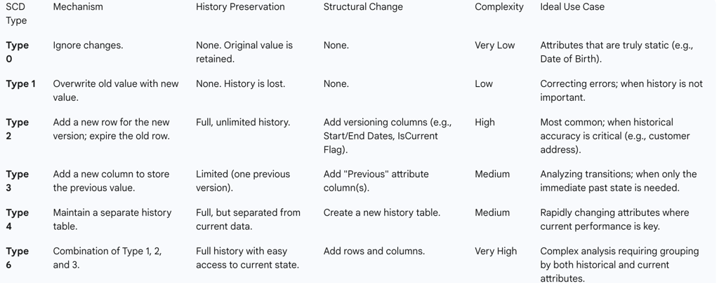
5.2 A Comprehensive Guide to SCD Types

Several standard methodologies exist for handling SCDs, each identified by a "Type" number.

5.2.1 Type 0: The Fixed Attribute (Retain Original)

This approach is used for attributes that are defined as fixed and should never change. Examples include a person's DateOfBirth or a product's OriginalLaunchDate. If a change to such an attribute is detected from a source system, it is treated as an error and is not applied to the dimension table.

5.2.2 Type 1: Overwrite

Type 1 is the simplest method. The old attribute value is directly overwritten with the new value, and no history of the change is preserved.

• Use Case: This method is appropriate only when historical accuracy for the attribute is not required. It is often used for correcting data entry errors (e.g., fixing a misspelled name) or for attributes where only the most current value is relevant (e.g., a customer's preferred contact phone number).

5.2.3 Type 2: Add New Row (Preserve Full History)

Type 2 is the most common, powerful, and widely used method for tracking historical changes. When a change occurs in a tracked attribute, the existing row is not overwritten. Instead, a new row is added to the dimension table to contain the new attribute values. The original row is "expired" or "closed out," typically by updating an EndDate column or setting an IsCurrent flag to false. The new row becomes the current, active record. This method requires a surrogate key to uniquely identify each version of the dimension member.

• Use Case: This is the standard for any attribute where historical context is critical for analysis, such as a customer's address, an employee's job title, or a product's category. It allows for perfect point-in-time reporting, ensuring that every fact is linked to the version of the dimension that was accurate at the time the fact occurred.

5.2.4 Type 3: Add New Column (Limited History)

The Type 3 method tracks a limited amount of history by adding a new column to the dimension table to store the "previous" value of an attribute. The main attribute column is overwritten with the new value (like Type 1), but the old value is preserved in the "previous value" column.

• Use Case: This is useful for situations where an analysis requires a direct comparison between the current and immediately prior state of an attribute, but a full history is not needed. For example, analyzing the impact of a sales territory realignment by comparing sales under the "Current Territory" and "Previous Territory" assignments. This method is not scalable for tracking more than one historical version.

5.2.5 Type 4: Add History Table

The Type 4 method involves creating two separate tables: a main dimension table that always stores only the current values (behaving like a Type 1 dimension), and a separate history table that archives all previous versions of the data.

• Use Case: This approach is often used for attributes that change very frequently, sometimes called "rapidly changing dimensions." Implementing a Type 2 approach for such attributes would cause the main dimension table to grow excessively large and slow down queries that only need the current state. By separating the current and historical data, performance for current-state queries is maintained, while the full history remains available for specialized analysis.

5.2.6 Type 6: Hybrid Approach

Type 6 is a hybrid technique that combines the methods of Type 1, Type 2, and Type 3 (as 1 + 2 + 3 = 6). When an attribute changes, it implements three actions simultaneously: a new row is added to preserve the full history (Type 2), the "current" attribute on the original row is overwritten with the new value to reflect the current state (Type 1), and a "historical" attribute column is maintained to track the value that was current for that version of the record (Type 3).

• Use Case: This advanced technique is used in complex analytical scenarios where analysts need the flexibility to group and filter historical facts by either the attribute value that was in effect at the time of the transaction or by the most current attribute value, without writing complex queries.

Table 4: Implementation Guide for Slowly Changing Dimensions

The Strategic Value of Dimensional Modeling in Business Intelligence

Dimensional modeling is more than a technical data structuring technique; it is a strategic framework that enables effective business intelligence and analytics. Its value is derived from a combination of performance optimization, enhanced usability for business users, and long-term flexibility.

6.1 Performance Optimization for Analytics

The simple, predictable structure of a dimensional model, particularly the star schema, is inherently optimized for the types of large-scale queries common in BI and analytics. The design minimizes the number of joins needed to connect facts with their context. Many relational database management systems have developed specific "star join" optimization algorithms that recognize this pattern and execute queries against it with exceptional efficiency. Furthermore, the use of denormalized dimension tables ensures that all the necessary contextual attributes for filtering and grouping are located in a single table, preventing the significant performance degradation that can occur when queries must navigate through multiple layers of normalized tables.

6.2 Usability and Accessibility for Business Users

A primary goal of dimensional modeling is to present data in a way that is intuitive and understandable to non-technical business users. The model achieves this by organizing data according to natural business processes and using familiar business terminology in table and column names. This business-centric design empowers a culture of self-service analytics. It allows business analysts and decision-makers to explore data, ask questions, and create reports using BI tools like Tableau or Power BI with minimal reliance on the IT department. These tools are often built around the dimensional paradigm, allowing users to easily "slice and dice" the data by dragging and dropping dimensional attributes to filter and group factual measures.

6.3 Flexibility and Extensibility

A well-designed dimensional model is highly resilient to change and can evolve gracefully as business requirements change. New quantitative measures can be added to a fact table as new columns without disrupting existing reports. New descriptive attributes can be added to dimension tables, becoming immediately available for analysis against all historical data. Entirely new dimensions can be associated with an existing fact table, as long as the grain of the fact table is respected. This extensibility allows the data warehouse to grow and adapt over time, protecting the initial investment and ensuring its long-term relevance to the organization.

While the historical impetus for dimensional modeling was often raw query performance on limited hardware, its enduring strategic value in the modern era has shifted. With the advent of powerful cloud data platforms and inexpensive compute, the most critical benefit is no longer just query speed. Instead, it is the model's ability to create a stable, reusable, and understandable "analytics layer" that fosters a common language between the technology teams and the business units. It functions as a governance and communication framework as much as a technical one. When an organization agrees on the definitions and hierarchies within a set of conformed dimensions, such as Dim_Product or Dim_Customer, it establishes a single, authoritative source of truth for core business concepts. This shared understanding prevents different departments from operating with conflicting data and definitions, ensuring that analytical results are consistent and trustworthy across the enterprise. The dimensional model, therefore, becomes the physical manifestation of an organization's shared business vocabulary, a crucial asset for fostering a data-driven culture.

Conclusion

This report has systematically deconstructed the core components and principles of dimensional modeling, the architectural bedrock of analytical data systems. The foundational dichotomy between quantitative facts and descriptive dimensions provides a powerful framework for organizing data in a manner that is both high-performing and business-intuitive. The choice of architectural schema—the simple, fast Star or the normalized, robust Snowflake—represents a critical trade-off between query speed and data integrity, a decision whose calculus is continually evolving with technology. Furthermore, the sophisticated techniques for managing temporal dynamics through Slowly Changing Dimensions are essential for preserving the historical accuracy that is the raison d'être of a data warehouse.

In the modern era of cloud data platforms like Snowflake, BigQuery, and Redshift, the relevance of these principles has not diminished. While the immense computational power of these systems has altered some of the historical performance considerations—lessening the strict need for pre-aggregation, for example—the fundamental logic of dimensional modeling remains as critical as ever. It provides the essential "staging layer" that transforms raw, often chaotic, source data into the clean, organized, and business-ready entities required by BI tools and data consumers. The dimensional model continues to be the most effective and proven methodology for designing data warehouses that deliver on their ultimate promise: to provide clear, consistent, and actionable insights from an organization's most valuable asset—its data.

Frequently Asked Questions

What is the difference between fact tables and dimension tables?

A fact table stores quantitative data for analysis, such as sales transactions, while a dimension table contains descriptive attributes, like customer demographics, that provide context for the facts1.

Can fact tables share dimension tables?

Yes, fact tables can share dimension tables, which is common in scenarios where conformed dimensions are used to ensure consistency across different datasets1.

What is a star and snowflake schema?

A star schema has a central fact table connected directly to flat dimension tables, while a snowflake schema normalizes dimension tables into additional tables to reduce redundancy1.

Are fact tables normalized or denormalized?

Fact tables are generally denormalized to optimize query performance, allowing for quicker data retrieval during analysis1.

What are the advantages of fact tables?

Fact tables allow for the storage of quantitative data, enabling aggregation and analysis to answer key business questions. They also connect to dimension tables for a more comprehensive understanding of the data1.

What is the difference between facts and dimensions in a star schema?

Facts represent measurable events (e.g., sales), while dimensions provide descriptive context (e.g., customer, product) for those facts in a star schema1.

Can a table be both fact and dimension?

Generally, tables are designated as either fact or dimension, but a table could theoretically serve both roles in different contexts, though this is uncommon and not a standard practice1.

Understanding the difference between fact and dimension tables is crucial for effective data modeling and designing a scalable data warehouse. By leveraging the strengths of both table types, you can transform raw data into actionable insights that drive business decisions.